Content-Based Analysis
Contents
Jaccard Index and Audio Features
Exploration of the Jaccard Index
In this part of the analysis, we explored the statistics of Jaccard index of the tracks in the dataset, and showed the importance of the Jaccard index as an indicator of similarity among songs.
First we import libraries and connect to the database.
import sqlite3
import pandas as pd
import numpy as np
import matplotlib
import matplotlib.pyplot as plt
%matplotlib inline

from math import factorial as fact
# create a new database by connecting to it
conn = sqlite3.connect("spotifyDB.db")
cur = conn.cursor()
# read the table to ensure that everything is working
pd.read_sql_query("select * from tracks WHERE num_member > 10 LIMIT 5;", conn)
| track | track_name | album | album_name | artist | artist_name | duration_ms | playlist_member | num_member | |
|---|---|---|---|---|---|---|---|---|---|
| 0 | 4HPBYMNnpP9Yc8u51VUyaD | Mariconatico | 5bZ7Jgk7YE35ULHWO3wgHP | Sincopa | 07PdYoE4jVRF6Ut40GgVSP | Cartel De Santa | 269333 | 1065,9003,10561,15769,21028,138066,147268,1567... | 11 |
| 1 | 3MCMHJ0p0tD0eRQC0Wg7Wu | Headshot! | 3k4aYVzOplQp6MTye2KlQ0 | Unbreakable | 4Uc6biA3i00oRAWvIfjhlk | MyChildren MyBride | 210813 | 3647,14323,35549,71836,74701,98691,113560,1189... | 13 |
| 2 | 2F950w5JasEsPPHfspO5yn | Know Your Onion - Spotify Sessions Curated by ... | 5aeSTpjqwuarRBM1zPCbOY | Spotify Sessions | 4LG4Bs1Gadht7TCrMytQUO | The Shins | 152653 | 2136,5176,27542,55583,77394,85407,118872,18360... | 11 |
| 3 | 5GAU7SP15OkPwj2tjXlUJn | Goodfriend | 2kyzu2gZ1SlkrzW6l4b7dD | Feathers & Fishhooks | 251UrhgNbMr15NLzQ2KyKq | Rayland Baxter | 266746 | 3626,8788,17107,49060,52900,53173,64212,66550,... | 15 |
| 4 | 7bTNGfXSJthLunBJzgOyBw | Harder | 5nL2ZC8NBSjMZfgpOp9P0w | FLYTRAP | 41yEdWozNYEzA2RfgYQHgr | CJ Fly | 177842 | 17432,30221,51929,53295,74242,86976,109832,139... | 11 |
# read the table
pd.read_sql_query("select * from playlists LIMIT 5;", conn)
| track | track_name | album | album_name | artist | artist_name | duration_ms | playlist_member | num_member | |
|---|---|---|---|---|---|---|---|---|---|
| 0 | 1Pm3fq1SC6lUlNVBGZi3Em | Concerning Hobbits (The Lord of the Rings) | 3q8vR3PFV8kG1m1Iv8DpKq | Versus Hollywood | 7zdmbPudNX4SQJXnYIuCTC | Daniel Tidwell | 108532 | 2 | 1 |
| 1 | 6BAwTzs5CWWuaaOpp6mTeL | End It Now! | 4SKnp9LlgXiEeVVud74fTS | Arrows | 4Xo1N4V7w6qX23OHAPcLCe | The Lonely Forest | 261146 | 4 | 1 |
| 2 | 3Ex4oMC0UeAQNAG78AuVfi | Pink City | 4ukM0IdJpt2NL8F8kDebS7 | A Promise | 5JLqvjW3Nyom2OsRUyFsS9 | Xiu Xiu | 133373 | 4 | 1 |
| 3 | 17q3q8wMWgYB8HoqZNNMRT | So Much Love So Little Time | 3jlchQb5BMfS7Cug5iceJn | Live A Little Love A Lot | 5juac7bFYyLKmV0VGSyaKM | Moose | 202533 | 4 | 1 |
| 4 | 6AAWJJ0zamfEVReLLDj4BC | Screaming | 5xxnHsOdealeAwAjfJfWH6 | . . . XYZ | 5juac7bFYyLKmV0VGSyaKM | Moose | 233733 | 4 | 1 |
| 5 | 1KVU56xCG8SqaXRjf9n4Da | Crush The Camera | 0ZvFi6ooJJOuMuMWfHAstk | 10:1 | 2JSc53B5cQ31m0xTB7JFpG | Rogue Wave | 180666 | 4 | 1 |
| 6 | 7331X4zR3C2eaLh5iHN98k | Interference | 5mmZbh9XqQaR0AEeevo5TS | Interference / Smile & Gesture | 3X03NfrYVLMXS2kz13t5WU | Lets Kill Janice | 212661 | 4 | 1 |
| 7 | 3O7HL3mzobCIxzErIMijxJ | Spread A Little Sunshine | 3Ll91eivgGYSJUVnL1WV4h | Playground | 3K6DKtqcjx8Vs5XEaTgZv7 | The Truth | 213466 | 4 | 1 |
| 8 | 5La66MFvn7AX8ZjXu2s8l8 | Kalte Wut / Wenn Ich Einmal Reich Bin | 6u6ISXvYPQkgzAQ170HUO0 | Lucky Streik | 04QGT0sr98LHIUjqPJ4RG4 | Floh de Cologne | 313066 | 4 | 1 |
| 9 | 3vUTaQZGXUTqgYWNUZiNW8 | Love's Been Good To Me | 27MGNEcpVfyejgypNIkogw | One by One | 62JorFOkIjXHHU7GMT9r77 | Rod McKuen | 183493 | 4 | 1 |
First of all, here we define functions that we will later use.
# this function creates all the unique pairwise combination of tracks within a playlist
def create_pair_from_playlist(playlist_id):
    query = 'SELECT tracks FROM playlists WHERE playlist_id = {};'.format(playlist_id)
    all_tracks = pd.read_sql_query(query, conn)
    ids = all_tracks['tracks'].values[0].split(',')
    track_pairs = [(track1, track2) for i, track1 in enumerate(ids)
               for j, track2 in enumerate(ids) if i<j]
    return track_pairs
# this function returns jaccard index between a pair of tracks (in tuple)
def similarity_btw_pair(pair_tuple):
    track_id1 = pair_tuple[0]
    track_id2 = pair_tuple[1]
    query = 'SELECT playlist_member, num_member FROM tracks WHERE track IN ("{}","{}");'.format(track_id1, track_id2)
    track_data = pd.read_sql_query(query, conn)

    mem1 = track_data['playlist_member'].values[0].split(',')
    mem2 = track_data['playlist_member'].values[1].split(',')
    num1 = track_data['num_member'].values[0]
    num2 = track_data['num_member'].values[1]
    # take intersect and union
    intersect = len(set(mem1).intersection(mem2))
    union = len(list(set(mem1) | set(mem1)))

    jaccard = intersect/union

    por1 = intersect/num1
    por2 = intersect/num2

    return jaccard, intersect, union, por1, por2
Jaccard index mean
We will pick 1000 different playlists, and then compute the mean Jaccard index from all the possible song combinations within each playlist.
Then, we will use the average number of songs within a playlist to pick random songs from the database, and thus find the mean Jaccard index for 1000 sets of random songs (not bootstrapped).
Here, we take 1000 random playlists:
# Pick 1000 random playlists
N = 1000

playlists = pd.read_sql_query('SELECT * FROM playlists ORDER BY RANDOM() LIMIT {};'.format(N), conn)
# How many songs per playlist?

mean_tracks = playlists[['num_tracks']].mean()
# Saving the jaccard means

# ATTENTION-- this cell takes hours to run.

jaccard_means = []

for i, playlist in playlists.iterrows():
    playlist_id = playlist.playlist_id
    track_pairs = create_pair_from_playlist(playlist_id)
    jaccard = []

    for pair_tuple in track_pairs:
        j,_,_,_,_ = similarity_btw_pair(pair_tuple)
        jaccard.append(j)

    jaccard = np.array(jaccard)
    jaccard_mean = np.mean(jaccard)

    jaccard_means.append(jaccard_mean)
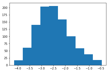
# Distribution of the LOG of the jaccard index means

plt.hist(np.log(jaccard_means));
plt.title('Jaccard Index- means for indices within playlists')
For the random playlists:
To find out how many random tracks we need to pick in order to explore the indices between random songs (instead of songs that exists in the same playlist), we need to compute the possible combinations of track from a 67 track playlist (67 an example mean size of a playlist), given by: \(\frac{n!}{(n-k)! k!}\) where n = 67 and k =2.
In order to create the random pairs from which the Jaccard indices will be calculated, we will pick twice that number of tracks, split the list of them into two, and then pair the two resulting lists up.
#For the number of random tracks:

mean_tracks_int = int(mean_tracks)

# Multiply by 2 because we intend to split the list
n_rand_tracks = int(2 *fact(mean_tracks_int)/(fact(mean_tracks_int-2)*fact(2)))
# Function that splits a list into two

def split_list(A):
    half = len(A)//2
    B = A[:half]
    C = A[half:]

    return B, C
# Find random tracks, make sure there's no duplicates, split list and join as tuples (ONLY ONE)

rand_tracks = pd.read_sql_query('SELECT track FROM tracks ORDER BY RANDOM() LIMIT {};'.format(n_rand_tracks), conn)
rand_tracks = list(set(rand_tracks[['track']].values[:,0]))

rand_list_a, rand_list_b = split_list(rand_tracks)
rand_tracks_paired = list(zip(rand_list_a, rand_list_b))
# Compute jaccard for one

jaccard_temp=[]
for pair in rand_tracks_paired:
    j_rand,_,_,_,_ = similarity_btw_pair(pair)
    jaccard_temp.append(j_rand)

jaccard_temp = np.array(jaccard_temp)
mean_pls = np.mean(jaccard_temp)
# Random tracks jaccard means

jaccard_rand_means = []
for i in range(N):
    rand_tracks = pd.read_sql_query('SELECT track FROM tracks ORDER BY RANDOM() LIMIT {};'.format(n_rand_tracks), conn)
    rand_tracks = list(set(rand_tracks[['track']].values[:,0]))

    rand_list_a, rand_list_b = split_list(rand_tracks)
    rand_tracks_paired = list(zip(rand_list_a, rand_list_b))

    jaccard_temp=[]
    for pair in rand_tracks_paired:
        j_rand,_,_,_,_ = similarity_btw_pair(pair)
        jaccard_temp.append(j_rand)

    jaccard_temp = np.array(jaccard_temp)
    mean_rand_jaccard = np.mean(jaccard_temp)

    jaccard_rand_means.append(mean_rand_jaccard)
    i += 1
# Plot

plt.figure(figsize = (10,7))
plt.title('Mean Jaccard index, N = {}'.format(N))
plt.hist(jaccard_means, label='Within  a playlist')
plt.hist(jaccard_rand_means, label='From random sample')
plt.xlabel('Jaccard index')
plt.ylabel('Frequency')
plt.legend()
<matplotlib.legend.Legend at 0x1a16925e48>
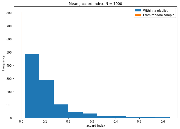
From this histogram, we see that there’s clearly two separate populations– the Jaccard index is much larger for songs that are ‘related’ (they’re together in playlists).
Content analysis: Can we predict a Jaccard index from audio features?
First of all, we can pick a random song, and explore what playlists it is in. Instead of just looking at the Jaccard index between it and a single playlist it is in, it would be more interesting to explore songs from ALL the playlists it is in, and then compare it to random songs.
Essentially, we will try to see if there’s a linear connection between the audio features of a song, and the Jaccard index between it and a random other song.
We are picking an equal distribution of random songs, and songs that populate the same playlists as the reference song, in order to ensure that there’s a distribution of Jaccard indices (given that most will hae an index of zero).
# First, pick a random track

track_EDA = pd.read_sql_query("SELECT * from tracks WHERE num_member > 3 ORDER BY RANDOM() LIMIT 1;", conn)
# Parse all the playlists for a single track:

track_EDA_playlists = track_EDA[['playlist_member']].values[0]
track_EDA_playlists = [x.strip() for x in track_EDA_playlists[0].split(',')]
track_EDA_playlists = [int(x) for x in track_EDA_playlists]
# Find all tracks that should have a higher Jaccard index from the playlists
EDA_ids = []
for playlist_id in track_EDA_playlists:
    query = 'SELECT tracks FROM playlists WHERE playlist_id = {};'.format(playlist_id)
    all_tracks = pd.read_sql_query(query, conn)
    ids = all_tracks['tracks'].values[0].split(',')
    EDA_ids.append(ids)

# Flatten the list
EDA_ids = [item for sublist in EDA_ids for item in sublist]

# Make unique and drop track
EDA_ids = list(set(EDA_ids))

track1 = track_EDA[['track']].values[0][0]

# Ensure that the tracks do NOT contain the track itself
EDA_ids.remove(track1)


# Make tuples

track_pairs_EDA = [(track1, track2) for track2 in EDA_ids]
# Between this song and random songs:

len_EDA = len(EDA_ids)

# Then pick the same number of songs

tracks_rand_EDA = pd.read_sql_query("SELECT * from tracks ORDER BY RANDOM() LIMIT {};".format(len_EDA), conn)
# Place the IDs of the random song into a list, and ensure only unique values

EDA_rand_ids = tracks_rand_EDA['track'].values.tolist()
EDA_rand_ids = list(set(EDA_rand_ids))

# Make sure the reference song itself is not in the playlist
try:
    EDA_rand_ids.remove(track1)
except:
    pass

# Concatenate lists
EDA_ids = EDA_ids+EDA_rand_ids

# Create tuples
track_pairs_EDA = [(track1, track2) for track2 in EDA_ids]
# Jaccard
jaccard_EDA = []

for pair_tuple in track_pairs_EDA:
    j_EDA,_,_,_,_ = similarity_btw_pair(pair_tuple)
    jaccard_EDA.append(j_EDA)
# Collect audio features:
import spotipy as sp
import spotipy.oauth2 as oauth2
import sqlite3
import pandas as pd

# set up authorization token
credentials = oauth2.SpotifyClientCredentials(

        client_id=='CLIENT_ID',
        client_secret='CLIENT_SECRET')

token = credentials.get_access_token()
spotify = sp.Spotify(auth=token)
# All audio features -- for regression purposes

danceability = []
energy = []
key = []
loudness = []
mode = []
speechiness = []
acousticness = []
instrumentalness = []
liveness = []
valence = []
tempo = []
duration_ms = []
time_signature = []

# Collect into lists:

for track_id in EDA_ids:
    results = spotify.audio_features(tracks=track_id)

    # Add into lists
    danceability.append(results[0]['danceability'])
    energy.append(results[0]['energy'])
    key.append(results[0]['key'])
    loudness.append(results[0]['loudness'])
    mode.append(results[0]['mode'])
    speechiness.append(results[0]['speechiness'])
    acousticness.append(results[0]['acousticness'])
    instrumentalness.append(results[0]['instrumentalness'])
    liveness.append(results[0]['liveness'])
    valence.append(results[0]['valence'])
    tempo.append(results[0]['tempo'])
    duration_ms.append(results[0]['duration_ms'])
    time_signature.append(results[0]['time_signature'])
# Create a dict, in order to make a pandas DataFrame
EDA_data = {}

EDA_data['ids']= EDA_ids
EDA_data['jaccard_EDA'] = jaccard_EDA

# Audio features
EDA_data['danceability']= danceability
EDA_data['energy']= energy
EDA_data['key']= key
EDA_data['loudness']= loudness
EDA_data['mode']= mode
EDA_data['speechiness']= speechiness
EDA_data['acousticness']= acousticness
EDA_data['instrumentalness']= instrumentalness
EDA_data['liveness']= liveness
EDA_data['valence']= valence
EDA_data['tempo']= tempo
EDA_data['duration_ms']= duration_ms
EDA_data['time_signature']= time_signature

EDA_results = pd.DataFrame.from_dict(EDA_data)
# Resulting pd:
EDA_results.head()
| ids | jaccard_EDA | danceability | energy | key | loudness | mode | speechiness | acousticness | instrumentalness | liveness | valence | tempo | duration_ms | time_signature | |
|---|---|---|---|---|---|---|---|---|---|---|---|---|---|---|---|
| 0 | 6pK6XXI3JHudVtl77QAfhh | 0.024390 | 0.547 | 0.395 | 0 | -9.654 | 0 | 0.0396 | 0.7850 | 0.000016 | 0.1240 | 0.697 | 140.992 | 197293 | 4 |
| 1 | 5BsOb3PMGwsMKTRpkabonh | 0.073171 | 0.655 | 0.692 | 6 | -11.728 | 1 | 0.0303 | 0.1640 | 0.000000 | 0.8210 | 0.668 | 111.253 | 183827 | 4 |
| 2 | 1dFITmhIit06htQ6dBRQOS | 0.500000 | 0.830 | 0.649 | 8 | -6.789 | 0 | 0.1510 | 0.0829 | 0.000220 | 0.0792 | 0.456 | 123.979 | 367960 | 4 |
| 3 | 7Lg5osturAd2VUP1rf0tEU | 0.024390 | 0.369 | 0.477 | 7 | -8.836 | 1 | 0.0354 | 0.7180 | 0.000037 | 0.1040 | 0.524 | 94.904 | 189213 | 4 |
| 4 | 27wLc0cxnw9IbhRMyMeBmR | 0.333333 | 0.775 | 0.553 | 1 | -10.512 | 1 | 0.0308 | 0.4850 | 0.842000 | 0.0453 | 0.820 | 120.005 | 286093 | 4 |
# Split into train and test sets
from sklearn.model_selection import train_test_split

# Response and independent variables:
X_vars = EDA_results[['danceability', 'energy', 'key', 'loudness', 'mode','speechiness', \
                      'acousticness','instrumentalness','liveness', 'valence', 'tempo', \
                      'duration_ms', 'time_signature']]

response = EDA_results[['jaccard_EDA']]

# Split:
Xtrain, Xtest, ytrain, ytest = train_test_split(X_vars,response,test_size=0.2)
Random Forest Regression using OOB
In order to do the regression, we can start with a random forest.
from sklearn.ensemble import RandomForestRegressor

# Code from lab 9, and:
# Adventures in scikit-learn's Random Forest by Gregory Saunders
from itertools import product
from collections import OrderedDict

param_dict = OrderedDict(
    n_estimators = [200, 400, 600, 800],
    max_features = [0.2, 0.4, 0.6, 0.8]
)

param_dict.values()
odict_values([[200, 400, 600, 800], [0.2, 0.4, 0.6, 0.8]])
from itertools import product
# Use Random Forest, and pick the best combination:
ytrain = np.ravel(ytrain)
RF_results = {}
RF_estimators = {}
for Ntrees, maxfeat in product(*param_dict.values()):
    params = (Ntrees, maxfeat)
    RF = RandomForestRegressor(oob_score=True,
                                n_estimators=Ntrees, max_features=maxfeat, max_depth=50)
    RF.fit(Xtrain, ytrain)
    RF_results[params] = RF.oob_score_
    RF_estimators[params] = RF
best_params = max(RF_results, key = RF_results.get)
best_params
(600, 0.2)
# Check accuracy
RF_final = RF_estimators[best_params]
print('The resulting accuracy from the RF is', RF_final.score(Xtest, ytest)*100, '%')
The resulting accuracy from the RF is 7.116939558688562 %
# Plot based on significance
pd.Series(RF_final.feature_importances_,index=list(Xtrain)).sort_values().plot(kind="barh")
This is very low accuracy, so regression does not seem too appealing. In any case, we can try a different method before rejecting the regression based on linearity.
Boosting
Last effort before rejecting this method will be boosting, using the “best predictors” from the previous analysis.
# Drop the worst predictors
ind_todrop = [index for index, value in enumerate(RF_final.feature_importances_) \
              if value < RF_final.score(Xtest, ytest)*0.5]

Xtrain_new = Xtrain.copy()

for ind in ind_todrop:
    col_todrop = Xtrain.columns[ind]
    Xtrain_new.drop(col_todrop, axis = 1)
We’re going to use the best parameters from the random forest eda
#Fit an Adaboost Model

from sklearn.ensemble import AdaBoostRegressor
from sklearn.tree import DecisionTreeRegressor

boosts = {}
boost_results = {}

for n in range(2,20):
    boost_model = AdaBoostRegressor(base_estimator=DecisionTreeRegressor(max_depth=n),\
                                    n_estimators=best_params[0],\
                                    learning_rate=0.05)
    boost_model.fit(Xtrain_new, ytrain)
    boosts[str(n)] = boost_model

    boost_results[str(n)] = boost_model.score(Xtest, ytest)
#Best depth accuracy

best_depth = max(boost_results, key = boost_results.get)
boost_final_score = boost_results[best_depth]

print('The best boosting model has a max_depth of {0} with a score of {1}%'.format(best_depth,100*boost_final_score))
The best boosting model has a max_depth of 11 with a score of 8.28111106007271%
This is stillnot a satisfactory accuracy score, which shows the need for both a different content-based analysis, and a collaborative filtering approach.
Making Song Recommendation with k-NN Clustering
Discovering similarities across Spotify tracks using clustering and audio features
We used Spotify’s audio features, such as acousticness and energy, to further analyze tracks and how these features impact users’ preferences, which in turn leads to users adding certain tracks to their playlists over others. Thus, we tried to explore how tracks and their audio features could potentially influence and be used to predict a user’s playlist preferences.
The k-NN model built below aims to cluster tracks based on their audio features. In order to perform feature selection for k-means clustering and to reduce the dimensionality of the feature space, we used Principal Component Analysis (PCA). Using PCA, we aimed to reduce the dimensionality of the data and identify the most important variables in the original feature space that contribute most to the variation in our data set. A dimension, or feature, that has not much variability cannot explain much of the happenings and thus, is not as important as more variable dimensions.
First we load the necessary libraries.
import sqlite3
import pandas as pd
import spotipy
import spotipy.oauth2 as oauth2
import pickle
import pandas.io.sql as psql
import numpy as np
from sklearn.preprocessing import StandardScaler
from sklearn.model_selection import train_test_split
from sklearn.decomposition import PCA
from sklearn.cluster import KMeans
import matplotlib
import matplotlib.pyplot as plt
%matplotlib inline
from sklearn.model_selection import GridSearchCV
from itertools import groupby
from operator import itemgetter
Load data
Here we connected to the Spotify SQL database, created an authorization token, and generated a list of 100 tracks by loading a pickle file that contains 171381 randomly-selected tracks from the Spotify Million Playlist dataset.
# connect to the database
conn = sqlite3.connect("spotifyDB.db")
c = conn.cursor()  # get a cursor
# set up authorization token
credentials = oauth2.SpotifyClientCredentials(
        client_id='CLIENT_ID',
        client_secret='CLIENT_SECRET')

token = credentials.get_access_token()
sp = spotipy.Spotify(auth=token)
c.execute("SELECT track FROM tracks")  # execute a simple SQL select query
jobs = c.fetchall()  # get all the results from the above query
with open('tracks_10000_rand.pkl', 'rb') as f:
    X = pickle.load(f)
Model Choice
We opted to use k-NN clustering by interpreting the numerical audio features as the distance between tracks because the advantage of using this algorithm is that it works on higher dimensions as well. As said above, to avoid the curse of dimensionality, we have nevertheless performed PCA and selected features that explain the majority of the variation of the dataset for k-means clustering. The k-NN works by finding the optimal number of clusters, k, and then defining k centroids (or points, which in our case are tracks) for each cluster. These centroids are then used to cluster the rest of the points, or tracks, into one of the k clusters.
Define functions
-
grouper This function allows to create a larger list of tracks to use for the clustering because Spotify limits how many times you can group into each of its API calls to 100 tracks.
-
process_features This function takes the list of dicts containing audio features for a number of tracks generated by accessing the Spotify API and converts it into a pandas dataframe.
# get the audio features of each of the tracks fetched above
track_features = {}
import itertools
def grouper(n, iterable):
    it = iter(iterable)
    while True:
        chunk = tuple(itertools.islice(it, n))
        if not chunk:
            return
        yield chunk

# can only take 100 songs at a time
for group in grouper(100, X[:1000]):
    track_features = sp.audio_features(tracks=group)

track_features
[{'danceability': 0.839,
  'energy': 0.791,
  'key': 8,
  'loudness': -7.771,
  'mode': 1,
  'speechiness': 0.116,
  'acousticness': 0.0531,
  'instrumentalness': 0.000485,
  'liveness': 0.201,
  'valence': 0.858,
  'tempo': 129.244,
  'type': 'audio_features',
  'id': '1YGa5zwwbzA9lFGPB3HcLt',
  'uri': 'spotify:track:1YGa5zwwbzA9lFGPB3HcLt',
  'track_href': 'https://api.spotify.com/v1/tracks/1YGa5zwwbzA9lFGPB3HcLt',
  'analysis_url': 'https://api.spotify.com/v1/audio-analysis/1YGa5zwwbzA9lFGPB3HcLt',
  'duration_ms': 267333,
  'time_signature': 4},
 {'danceability': 0.728,
  'energy': 0.779,
  'key': 4,
  'loudness': -7.528,
  'mode': 0,
  'speechiness': 0.19,
  'acousticness': 0.00336,
  'instrumentalness': 1.18e-06,
  'liveness': 0.325,
  'valence': 0.852,
  'tempo': 174.046,
  'type': 'audio_features',
  'id': '4gOMf7ak5Ycx9BghTCSTBL',
  'uri': 'spotify:track:4gOMf7ak5Ycx9BghTCSTBL',
  'track_href': 'https://api.spotify.com/v1/tracks/4gOMf7ak5Ycx9BghTCSTBL',
  'analysis_url': 'https://api.spotify.com/v1/audio-analysis/4gOMf7ak5Ycx9BghTCSTBL',
  'duration_ms': 278810,
  'time_signature': 4},

 {'danceability': 0.541,
  'energy': 0.748,
  'key': 2,
  'loudness': -6.321,
  'mode': 1,
  'speechiness': 0.31,
  'acousticness': 0.00141,
  'instrumentalness': 3.1e-06,
  'liveness': 0.322,
  'valence': 0.351,
  'tempo': 79.616,
  'type': 'audio_features',
  'id': '1rW2nkUbmKD2MC22YrU8cX',
  'uri': 'spotify:track:1rW2nkUbmKD2MC22YrU8cX',
  'track_href': 'https://api.spotify.com/v1/tracks/1rW2nkUbmKD2MC22YrU8cX',
  'analysis_url': 'https://api.spotify.com/v1/audio-analysis/1rW2nkUbmKD2MC22YrU8cX',
  'duration_ms': 196427,
  'time_signature': 4}]
# populate the tracks feature dataframe
def process_features(features_list_dicts):
    features_df = pd.DataFrame(features_list_dicts)
    features_df = features_df.set_index('id')
    return features_df

features_df=process_features(track_features)
features_df.head()
| acousticness | analysis_url | danceability | duration_ms | energy | instrumentalness | key | liveness | loudness | mode | speechiness | tempo | time_signature | track_href | type | uri | valence | |
|---|---|---|---|---|---|---|---|---|---|---|---|---|---|---|---|---|---|
| id | |||||||||||||||||
| 1YGa5zwwbzA9lFGPB3HcLt | 0.05310 | https://api.spotify.com/v1/audio-analysis/1YGa... | 0.839 | 267333 | 0.791 | 0.000485 | 8 | 0.2010 | -7.771 | 1 | 0.1160 | 129.244 | 4 | https://api.spotify.com/v1/tracks/1YGa5zwwbzA9... | audio_features | spotify:track:1YGa5zwwbzA9lFGPB3HcLt | 0.858 |
| 4gOMf7ak5Ycx9BghTCSTBL | 0.00336 | https://api.spotify.com/v1/audio-analysis/4gOM... | 0.728 | 278810 | 0.779 | 0.000001 | 4 | 0.3250 | -7.528 | 0 | 0.1900 | 174.046 | 4 | https://api.spotify.com/v1/tracks/4gOMf7ak5Ycx... | audio_features | spotify:track:4gOMf7ak5Ycx9BghTCSTBL | 0.852 |
| 7kl337nuuTTVcXJiQqBgwJ | 0.44700 | https://api.spotify.com/v1/audio-analysis/7kl3... | 0.314 | 451160 | 0.855 | 0.854000 | 2 | 0.1730 | -7.907 | 1 | 0.0340 | 104.983 | 4 | https://api.spotify.com/v1/tracks/7kl337nuuTTV... | audio_features | spotify:track:7kl337nuuTTVcXJiQqBgwJ | 0.855 |
| 0LAfANg75hYiV1IAEP3vY6 | 0.22000 | https://api.spotify.com/v1/audio-analysis/0LAf... | 0.762 | 271907 | 0.954 | 0.000018 | 8 | 0.0612 | -4.542 | 1 | 0.1210 | 153.960 | 4 | https://api.spotify.com/v1/tracks/0LAfANg75hYi... | audio_features | spotify:track:0LAfANg75hYiV1IAEP3vY6 | 0.933 |
| 0Hpl422q9VhpQu1RBKlnF1 | 0.42200 | https://api.spotify.com/v1/audio-analysis/0Hpl... | 0.633 | 509307 | 0.834 | 0.726000 | 11 | 0.1720 | -12.959 | 1 | 0.0631 | 130.008 | 4 | https://api.spotify.com/v1/tracks/0Hpl422q9Vhp... | audio_features | spotify:track:0Hpl422q9VhpQu1RBKlnF1 | 0.518 |
** NOTE: ** We created a pandas dataframe called features_df_updated that includes only the numerical audio features of the selected tracks to perform PCA later on.
# drop the non-numerical columns
features_df_updated = features_df.drop(['analysis_url', 'track_href', 'type', 'uri' ], axis=1)
features_df_updated.head()
| acousticness | danceability | duration_ms | energy | instrumentalness | key | liveness | loudness | mode | speechiness | tempo | time_signature | valence | |
|---|---|---|---|---|---|---|---|---|---|---|---|---|---|
| id | |||||||||||||
| 1YGa5zwwbzA9lFGPB3HcLt | 0.05310 | 0.839 | 267333 | 0.791 | 0.000485 | 8 | 0.2010 | -7.771 | 1 | 0.1160 | 129.244 | 4 | 0.858 |
| 4gOMf7ak5Ycx9BghTCSTBL | 0.00336 | 0.728 | 278810 | 0.779 | 0.000001 | 4 | 0.3250 | -7.528 | 0 | 0.1900 | 174.046 | 4 | 0.852 |
| 7kl337nuuTTVcXJiQqBgwJ | 0.44700 | 0.314 | 451160 | 0.855 | 0.854000 | 2 | 0.1730 | -7.907 | 1 | 0.0340 | 104.983 | 4 | 0.855 |
| 0LAfANg75hYiV1IAEP3vY6 | 0.22000 | 0.762 | 271907 | 0.954 | 0.000018 | 8 | 0.0612 | -4.542 | 1 | 0.1210 | 153.960 | 4 | 0.933 |
| 0Hpl422q9VhpQu1RBKlnF1 | 0.42200 | 0.633 | 509307 | 0.834 | 0.726000 | 11 | 0.1720 | -12.959 | 1 | 0.0631 | 130.008 | 4 | 0.518 |
Store data into SQL database
We decided to generate SQL tables to store and manipulate our tracks data.
-
track_features This SQL table stores all the numerical audio features for a list of tracks that will be used to perform PCA and k-means clustering.
-
BigTable This SQL table is generated by inner joining the previously generated tracks table with the track_features table on the track ID. This table comes in handy after we cluster the list of tracks to get more details about the tracks in each cluster, not just the track ID (i.e. the track name, playlists it appears in, album name, artist name etc.)
# create the tracks feature table
query = 'DROP TABLE IF EXISTS track_features;'
c.execute(query)
conn.commit()

c.execute('''CREATE TABLE IF NOT EXISTS track_features (id varchar(255) PRIMARY KEY,
         acousticness integer,danceability integer, duration_ms integer, energy integer,
         instrumentalness integer, key integer, liveness integer, loudness integer,
         mode integer, speechiness integer, tempo integer, time_signature integer,
         valence integer
         );''')
conn.commit()
# insert track features dataframe into track features SQL table
features_df_updated.to_sql('track_features', conn, if_exists='append')
# read the track features table
pd.read_sql_query("select * from track_features LIMIT 10;", conn)
| id | acousticness | danceability | duration_ms | energy | instrumentalness | key | liveness | loudness | mode | speechiness | tempo | time_signature | valence | |
|---|---|---|---|---|---|---|---|---|---|---|---|---|---|---|
| 0 | 1YGa5zwwbzA9lFGPB3HcLt | 0.05310 | 0.839 | 267333 | 0.791 | 0.000485 | 8 | 0.2010 | -7.771 | 1 | 0.1160 | 129.244 | 4 | 0.858 |
| 1 | 4gOMf7ak5Ycx9BghTCSTBL | 0.00336 | 0.728 | 278810 | 0.779 | 0.000001 | 4 | 0.3250 | -7.528 | 0 | 0.1900 | 174.046 | 4 | 0.852 |
| 2 | 7kl337nuuTTVcXJiQqBgwJ | 0.44700 | 0.314 | 451160 | 0.855 | 0.854000 | 2 | 0.1730 | -7.907 | 1 | 0.0340 | 104.983 | 4 | 0.855 |
| 3 | 0LAfANg75hYiV1IAEP3vY6 | 0.22000 | 0.762 | 271907 | 0.954 | 0.000018 | 8 | 0.0612 | -4.542 | 1 | 0.1210 | 153.960 | 4 | 0.933 |
| 4 | 0Hpl422q9VhpQu1RBKlnF1 | 0.42200 | 0.633 | 509307 | 0.834 | 0.726000 | 11 | 0.1720 | -12.959 | 1 | 0.0631 | 130.008 | 4 | 0.518 |
| 5 | 4uTTsXhygWzSjUxXLHZ4HW | 0.12600 | 0.724 | 231824 | 0.667 | 0.000000 | 4 | 0.1220 | -4.806 | 0 | 0.3850 | 143.988 | 4 | 0.161 |
| 6 | 1KDnLoIEPRd4iRYzgvDBzo | 0.22100 | 0.617 | 259147 | 0.493 | 0.294000 | 0 | 0.6960 | -12.779 | 1 | 0.0495 | 119.003 | 4 | 0.148 |
| 7 | 0j9rNb4IHxLgKdLGZ1sd1I | 0.43500 | 0.353 | 407814 | 0.304 | 0.000002 | 4 | 0.8020 | -9.142 | 0 | 0.0327 | 138.494 | 4 | 0.233 |
| 8 | 1Dfst5fQZYoW8QBfo4mUmn | 0.22100 | 0.633 | 205267 | 0.286 | 0.004150 | 2 | 0.0879 | -9.703 | 0 | 0.0270 | 129.915 | 4 | 0.196 |
| 9 | 6ZbiaHwI9x7CIxYGOEmXxd | 0.56400 | 0.569 | 198012 | 0.789 | 0.000000 | 11 | 0.2940 | -4.607 | 1 | 0.1230 | 160.014 | 4 | 0.603 |
query = 'DROP TABLE IF EXISTS BigTable;'
c.execute(query)
conn.commit()

c.execute(""" CREATE TABLE BigTable AS
            SELECT tracks.track,tracks.track_name, tracks.album, tracks.album_name, tracks.artist,
            tracks.artist_name, tracks.duration_ms, tracks.playlist_member, tracks.num_member,
            track_features.acousticness,track_features.danceability, track_features.energy,
            track_features.instrumentalness,track_features.key, track_features.liveness,track_features.loudness,
            track_features.mode, track_features.speechiness, track_features.tempo, track_features.time_signature,
            track_features.valence
            FROM tracks
            INNER JOIN track_features
            ON tracks.track = track_features.id""")
<sqlite3.Cursor at 0x1a1410d1f0>
# create SQL table containing both qualitative and quantitative information about tracks
tracks_merged_df = psql.read_sql_query("SELECT * from BigTable ", conn)
tracks_merged_df.head()
| track | track_name | album | album_name | artist | artist_name | duration_ms | playlist_member | num_member | acousticness | ... | energy | instrumentalness | key | liveness | loudness | mode | speechiness | tempo | time_signature | valence | |
|---|---|---|---|---|---|---|---|---|---|---|---|---|---|---|---|---|---|---|---|---|---|
| 0 | 1YGa5zwwbzA9lFGPB3HcLt | Suavemente - Spanglish Edit | 6hGJXv2n5dNuIpaxpgSBOe | Suavemente, The Remixes | 1c22GXH30ijlOfXhfLz9Df | Elvis Crespo | 267333 | 92453,112168,121648,238345,245267,303554,31985... | 12 | 0.05310 | ... | 0.791 | 0.000485 | 8 | 0.2010 | -7.771 | 1 | 0.1160 | 129.244 | 4 | 0.858 |
| 1 | 4gOMf7ak5Ycx9BghTCSTBL | Sexo X Money (feat. Ozuna) | 3BB6mEEVz8vb2yMRSPHiDR | 8 Semanas | 5gUZ67Vzi1FV2SnrWl1GlE | Benny Benni | 278809 | 96862,117960 | 2 | 0.00336 | ... | 0.779 | 0.000001 | 4 | 0.3250 | -7.528 | 0 | 0.1900 | 174.046 | 4 | 0.852 |
| 2 | 7kl337nuuTTVcXJiQqBgwJ | Jessica - Unedited Version | 1n9rbMLUmrXBBBJffS7pDj | Brothers And Sisters | 4wQ3PyMz3WwJGI5uEqHUVR | The Allman Brothers Band | 451160 | 1231,2588,3054,4223,4777,4955,5094,5199,5991,6... | 871 | 0.44700 | ... | 0.855 | 0.854000 | 2 | 0.1730 | -7.907 | 1 | 0.0340 | 104.983 | 4 | 0.855 |
| 3 | 0LAfANg75hYiV1IAEP3vY6 | Take Your Mama | 65Fllu4vQdZQOh6id0YwIM | Scissor Sisters | 3Y10boYzeuFCJ4Qgp53w6o | Scissor Sisters | 271906 | 1697,2647,3150,5142,5199,6597,6669,7301,7367,7... | 534 | 0.22000 | ... | 0.954 | 0.000018 | 8 | 0.0612 | -4.542 | 1 | 0.1210 | 153.960 | 4 | 0.933 |
| 4 | 0Hpl422q9VhpQu1RBKlnF1 | 3rd Chakra "Sacred Fire" | 07fAo1agwL9nuky8VmMhNa | Chakradance | 3kbO7dxGm5uux3yrXYlnvR | Jonthan Goldman | 509306 | 231516 | 1 | 0.42200 | ... | 0.834 | 0.726000 | 11 | 0.1720 | -12.959 | 1 | 0.0631 | 130.008 | 4 | 0.518 |
5 rows × 21 columns
pd.read_sql_query("SELECT * from BigTable ", conn)
| track | track_name | album | album_name | artist | artist_name | duration_ms | playlist_member | num_member | acousticness | ... | energy | instrumentalness | key | liveness | loudness | mode | speechiness | tempo | time_signature | valence | |
|---|---|---|---|---|---|---|---|---|---|---|---|---|---|---|---|---|---|---|---|---|---|
| 0 | 1YGa5zwwbzA9lFGPB3HcLt | Suavemente - Spanglish Edit | 6hGJXv2n5dNuIpaxpgSBOe | Suavemente, The Remixes | 1c22GXH30ijlOfXhfLz9Df | Elvis Crespo | 267333 | 92453,112168,121648,238345,245267,303554,31985... | 12 | 0.053100 | ... | 0.791 | 0.000485 | 8 | 0.2010 | -7.771 | 1 | 0.1160 | 129.244 | 4 | 0.8580 |
| 1 | 4gOMf7ak5Ycx9BghTCSTBL | Sexo X Money (feat. Ozuna) | 3BB6mEEVz8vb2yMRSPHiDR | 8 Semanas | 5gUZ67Vzi1FV2SnrWl1GlE | Benny Benni | 278809 | 96862,117960 | 2 | 0.003360 | ... | 0.779 | 0.000001 | 4 | 0.3250 | -7.528 | 0 | 0.1900 | 174.046 | 4 | 0.8520 |
| 2 | 7kl337nuuTTVcXJiQqBgwJ | Jessica - Unedited Version | 1n9rbMLUmrXBBBJffS7pDj | Brothers And Sisters | 4wQ3PyMz3WwJGI5uEqHUVR | The Allman Brothers Band | 451160 | 1231,2588,3054,4223,4777,4955,5094,5199,5991,6... | 871 | 0.447000 | ... | 0.855 | 0.854000 | 2 | 0.1730 | -7.907 | 1 | 0.0340 | 104.983 | 4 | 0.8550 |
| 3 | 0LAfANg75hYiV1IAEP3vY6 | Take Your Mama | 65Fllu4vQdZQOh6id0YwIM | Scissor Sisters | 3Y10boYzeuFCJ4Qgp53w6o | Scissor Sisters | 271906 | 1697,2647,3150,5142,5199,6597,6669,7301,7367,7... | 534 | 0.220000 | ... | 0.954 | 0.000018 | 8 | 0.0612 | -4.542 | 1 | 0.1210 | 153.960 | 4 | 0.9330 |
| 4 | 0Hpl422q9VhpQu1RBKlnF1 | 3rd Chakra "Sacred Fire" | 07fAo1agwL9nuky8VmMhNa | Chakradance | 3kbO7dxGm5uux3yrXYlnvR | Jonthan Goldman | 509306 | 231516 | 1 | 0.422000 | ... | 0.834 | 0.726000 | 11 | 0.1720 | -12.959 | 1 | 0.0631 | 130.008 | 4 | 0.5180 |
| 5 | 4uTTsXhygWzSjUxXLHZ4HW | No Way | 1ST1X21yXzG5rJtflnBXFT | The Rise | 5Z5jUyiNvFaqp0EVyLNf0p | Futuristic | 231823 | 1198,2027,3511,5700,6087,6472,9139,10313,12001... | 243 | 0.126000 | ... | 0.667 | 0.000000 | 4 | 0.1220 | -4.806 | 0 | 0.3850 | 143.988 | 4 | 0.1610 |
| 6 | 1KDnLoIEPRd4iRYzgvDBzo | Far Away Place | 3bcrjy1PXm8vwbqP6ylr6j | On The Quiet | 1w7cucUEPR1Yq9g03g6T8m | Xinobi | 259146 | 460,11131,13976,24479,27781,31117,34279,35995,... | 70 | 0.221000 | ... | 0.493 | 0.294000 | 0 | 0.6960 | -12.779 | 1 | 0.0495 | 119.003 | 4 | 0.1480 |
100 rows × 21 columns
Preparing the Data for k-NN Clustering
Scaling the Features
- scale_datasets This function scales a set of variables from the data set, which will then be used for k-NN clustering. In our case, we dealt with mixed numerical features that had different units attached, so to ensure comparability across these features, we standardized our numerical audio features.
NOTE: Because we also had some categorical and non-numerical variables in our dataset, we specifically defined the numerical features to be scaled.
train_tracks = tracks_merged_df
def scale_datasets(train_data, cols_to_scale):
    train = train_data.copy()
    # fit the scaler on the training data
    scaler = StandardScaler().fit(train[cols_to_scale])
    # scale both the test and training data.
    train[cols_to_scale] = scaler.transform(train[cols_to_scale])
    return train

# get columns that need to be scaled
not_to_scale = ['mode', 'track', 'track_name', 'album', 'album_name', 'artist', 'artist_name', 'playlist_member']
to_scale = train_tracks.columns.difference(not_to_scale)
# train_tracks_scaled, test_tracks_scaled = scale_datasets(train_tracks, test_tracks, to_scale)
train_tracks_scaled = scale_datasets(train_tracks, to_scale)
train_tracks_scaled.describe()
/Users/andrafehmiu/Desktop/anaconda3/lib/python3.6/site-packages/sklearn/preprocessing/data.py:617: DataConversionWarning: Data with input dtype int64, float64 were all converted to float64 by StandardScaler.
  return self.partial_fit(X, y)
/Users/andrafehmiu/Desktop/anaconda3/lib/python3.6/site-packages/ipykernel_launcher.py:6: DataConversionWarning: Data with input dtype int64, float64 were all converted to float64 by StandardScaler.
| duration_ms | num_member | acousticness | danceability | energy | instrumentalness | key | liveness | loudness | mode | speechiness | tempo | time_signature | valence | |
|---|---|---|---|---|---|---|---|---|---|---|---|---|---|---|
| count | 1.000000e+02 | 1.000000e+02 | 1.000000e+02 | 1.000000e+02 | 1.000000e+02 | 1.000000e+02 | 1.000000e+02 | 1.000000e+02 | 1.000000e+02 | 100.000000 | 1.000000e+02 | 1.000000e+02 | 1.000000e+02 | 1.000000e+02 |
| mean | 3.552714e-17 | -1.998401e-17 | -1.865175e-16 | -3.019807e-16 | -9.248158e-16 | 3.108624e-17 | 6.328271e-17 | 5.995204e-17 | 4.551914e-17 | 0.690000 | -3.153033e-16 | -2.797762e-16 | 5.717649e-17 | -1.815215e-16 |
| std | 1.005038e+00 | 1.005038e+00 | 1.005038e+00 | 1.005038e+00 | 1.005038e+00 | 1.005038e+00 | 1.005038e+00 | 1.005038e+00 | 1.005038e+00 | 0.464823 | 1.005038e+00 | 1.005038e+00 | 1.005038e+00 | 1.005038e+00 |
| min | -1.728999e+00 | -2.673091e-01 | -9.338852e-01 | -2.979480e+00 | -2.544541e+00 | -3.706251e-01 | -1.303501e+00 | -8.787226e-01 | -3.447685e+00 | 0.000000 | -7.794134e-01 | -2.251437e+00 | -7.450531e+00 | -1.612685e+00 |
| 25% | -4.968337e-01 | -2.599727e-01 | -8.631080e-01 | -5.617366e-01 | -6.800231e-01 | -3.706251e-01 | -1.031938e+00 | -6.307094e-01 | -5.163343e-01 | 0.000000 | -6.611387e-01 | -7.300483e-01 | 2.041241e-01 | -8.828781e-01 |
| 50% | -1.783776e-01 | -2.350289e-01 | -3.411226e-01 | 2.007501e-01 | 3.261311e-01 | -3.705485e-01 | -2.172502e-01 | -4.567182e-01 | 6.166226e-02 | 1.000000 | -4.868391e-01 | 3.691746e-02 | 2.041241e-01 | -1.652379e-01 |
| 75% | 3.350748e-01 | -1.396557e-01 | 6.116665e-01 | 7.185807e-01 | 6.666392e-01 | -3.525086e-01 | 8.690007e-01 | 4.099448e-01 | 7.721308e-01 | 1.000000 | 2.420501e-01 | 6.311570e-01 | 2.041241e-01 | 8.271018e-01 |
| max | 6.518389e+00 | 8.075645e+00 | 2.507656e+00 | 1.899835e+00 | 1.503722e+00 | 3.295369e+00 | 1.683689e+00 | 3.924013e+00 | 1.718260e+00 | 1.000000 | 3.442258e+00 | 2.616494e+00 | 2.755676e+00 | 1.802332e+00 |
Feature Selection Using PCA
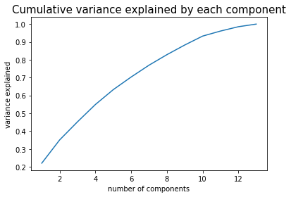
- pca_x This function performs PCA on a given set of features and allows to tune the maximum number of PCs and the percent of variation in data set that we want the PCs to explain. It also generates a plot of cumulative variance explained by a given number of PCs up to the maximum number of PCs that is fed into the function.
In our case, we decided to use a threshold of 0.9 for the threshold variation and we picked the number of features accordingly based on the number required to explain at least 90% of the variation in the original data set, which turned out to be 10 PCs.
- optimal_pca This function generates training data containing only the optimal/most important features– in our case, the number of optimal features was determined after generating the plot of cumulative variance explained by each PC from the pca_x function.
def pca_x(data_train, to_scale, total_comp, var_thresh):
    data_train = data_train.set_index('track')
    train_tracks_copy = data_train[to_scale].copy()
    # applying PCA
    pca = PCA(n_components= total_comp) # from our result in 1.5
    pca.fit(train_tracks_copy)
    # transforming train data
    x_train_pca = pca.transform(train_tracks_copy)
    # plot pca var explained as function of number of PCs
    plt.plot(np.linspace(1, total_comp, total_comp), np.cumsum(pca.explained_variance_ratio_))
    plt.xlabel('number of components')
    plt.ylabel('variance explained')
    plt.title('Cumulative variance explained by each component',fontsize=15)
    optimal = np.where(np.cumsum(pca.explained_variance_ratio_)<=var_thresh)[0]+1
    return x_train_pca

x_train_pca = pca_x(train_tracks_scaled, to_scale, 13, 0.9)
def optimal_pca(data_train, to_scale, optimal_comp):
    data_train = data_train.set_index('track')
    train_tracks_copy = data_train[to_scale].copy()
    # applying PCA
    pca = PCA(n_components= optimal_comp) # from our result in 1.5
    pca.fit(train_tracks_copy)
    # transforming data
    optimal_x_pca = pca.transform(train_tracks_copy)
    return optimal_x_pca

optimal_x_pca = optimal_pca(train_tracks_scaled, to_scale, 10)
Clustering the 100 randomly selected tracks across different playlists
After pre-processing our features data via scaling and PCA, we processed with the clustering of the 100 randomly-selected tracks across playlists based on the similiarity of the most important features, i.e. the ones that cumulatively explain about 90% of the variation of the data set.
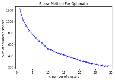
- knn_clustering This function fits the training data, calculates the distance between each track as (where the audio features are interpreted as “distances” between tracks), and generates an elbow plot that is helpful to determine k, the optimal number of clusters to be used in our model.
def knn_clustering(pca_train, k_train):
    knn_sum_squared_distances_train = []
    for k in k_train:
        knn_train = KMeans(n_clusters= k)
        knn_train = knn_train.fit(pca_train)
        knn_sum_squared_distances_train.append(knn_train.inertia_)
    plt.plot(k_train, knn_sum_squared_distances_train, 'bx-')
    plt.xlabel('k, number of clusters')
    plt.ylabel('Sum of squared distances')
    plt.title('Elbow Method For Optimal k')
    plt.show()
    return knn_sum_squared_distances_train
k_train = range(1, 30)
cluster_optimal = knn_clustering(optimal_x_pca, k_train)
print(cluster_optimal[10:20])
cluster_optimal[15]
[508.29601759835464, 478.66012661207566, 455.42988212581963, 433.1924769385507, 405.0390458655179, 394.42230803397507, 376.5035667562909, 354.1919104711137, 337.52153447950127, 324.3814147730095]


394.42230803397507
Generating Optimal k-NN Clusters
- optimal_knn_clustering This function clusters the tracks into k clusters, where k in our case was determined based on the elbow plot generated by the knn_clustering function above.
We decided to classify our tracks into 15 clusters by using the elbow plot and observing that 15 clusters significantly reduce the sum of squared distances between tracks while also providing a sensible model. I.e. choosing 100 clusters would simply mean that each track would be the centroid and also the only point in the cluster and although the sume of the squared distance would be 0, the model itself wouldn’t be useful in determining the similarity of tracks.
# based on the elbow plot, we pick k number of cluster to be 15
def optimal_knn_clustering(pca_train, k):
        knn_sum_squared_distances_train=[]
        knn_train = KMeans(n_clusters= k)
        knn_train = knn_train.fit(pca_train)
        # predict clusters
        labels = knn_train.predict(pca_train)
        # get cluster centers
        centers = knn_train.cluster_centers_
        return labels, centers

clusters, centers = optimal_knn_clustering(optimal_x_pca, 15)
clusters
array([ 2, 13,  6,  2,  6, 11, 10, 10, 10,  2,  2,  3,  0,  0, 13, 10,  6,
        5,  7, 13, 10,  9,  5,  1, 10,  9,  1,  4,  0, 11,  2,  2, 10,  8,
        8, 11, 10, 12,  1, 10,  8,  5,  2,  2,  2, 10,  1, 10,  2,  1,  1,
        1,  2, 10,  6,  1,  1,  5,  5, 13,  1,  6,  5,  5, 11,  5,  8, 13,
        2, 13, 11, 11,  8,  2, 14, 11,  5,  1, 11,  1,  6,  2, 13,  1,  2,
        1, 10, 10,  2,  1,  2,  8,  3,  1,  8,  2,  1,  1, 13, 11],
      dtype=int32)
k-NN Clustering Conclusion
Based on the k-nn clustering model, we can see that the clusters obtained make sense intuitevely – i.e. songs such as Suavement and Take Your Mama are clustered together – which having listened to these songs make sense as they do sound similiar without an-indepth analysis of their audio features. An interesting thing to note is that on a few occassions, re-running the k-NN clustering led to different clustering of these tracks, which indicates the instability of this model, which could be caused by the fact that the tracks to be clustered might be similar to more than one of the centroids of the k clusters. Thus, this model manages to cluster tracks based on their audio features’ similarity, but is not the most robust and hence, is not the optimal model.
train_tracks['predicted cluster label'] = clusters.tolist()
train_tracks
| track | track_name | album | album_name | artist | artist_name | duration_ms | playlist_member | num_member | acousticness | ... | instrumentalness | key | liveness | loudness | mode | speechiness | tempo | time_signature | valence | predicted cluster label | |
|---|---|---|---|---|---|---|---|---|---|---|---|---|---|---|---|---|---|---|---|---|---|
| 0 | 1YGa5zwwbzA9lFGPB3HcLt | Suavemente - Spanglish Edit | 6hGJXv2n5dNuIpaxpgSBOe | Suavemente, The Remixes | 1c22GXH30ijlOfXhfLz9Df | Elvis Crespo | 267333 | 92453,112168,121648,238345,245267,303554,31985... | 12 | 0.053100 | ... | 0.000485 | 8 | 0.2010 | -7.771 | 1 | 0.1160 | 129.244 | 4 | 0.8580 | 2 |
| 1 | 4gOMf7ak5Ycx9BghTCSTBL | Sexo X Money (feat. Ozuna) | 3BB6mEEVz8vb2yMRSPHiDR | 8 Semanas | 5gUZ67Vzi1FV2SnrWl1GlE | Benny Benni | 278809 | 96862,117960 | 2 | 0.003360 | ... | 0.000001 | 4 | 0.3250 | -7.528 | 0 | 0.1900 | 174.046 | 4 | 0.8520 | 13 |
| 2 | 7kl337nuuTTVcXJiQqBgwJ | Jessica - Unedited Version | 1n9rbMLUmrXBBBJffS7pDj | Brothers And Sisters | 4wQ3PyMz3WwJGI5uEqHUVR | The Allman Brothers Band | 451160 | 1231,2588,3054,4223,4777,4955,5094,5199,5991,6... | 871 | 0.447000 | ... | 0.854000 | 2 | 0.1730 | -7.907 | 1 | 0.0340 | 104.983 | 4 | 0.8550 | 6 |
| 3 | 0LAfANg75hYiV1IAEP3vY6 | Take Your Mama | 65Fllu4vQdZQOh6id0YwIM | Scissor Sisters | 3Y10boYzeuFCJ4Qgp53w6o | Scissor Sisters | 271906 | 1697,2647,3150,5142,5199,6597,6669,7301,7367,7... | 534 | 0.220000 | ... | 0.000018 | 8 | 0.0612 | -4.542 | 1 | 0.1210 | 153.960 | 4 | 0.9330 | 2 |
| 4 | 0Hpl422q9VhpQu1RBKlnF1 | 3rd Chakra "Sacred Fire" | 07fAo1agwL9nuky8VmMhNa | Chakradance | 3kbO7dxGm5uux3yrXYlnvR | Jonthan Goldman | 509306 | 231516 | 1 | 0.422000 | ... | 0.726000 | 11 | 0.1720 | -12.959 | 1 | 0.0631 | 130.008 | 4 | 0.5180 | 6 |
100 rows × 22 columns